A MORPHEUS PRODUCTION
MULTIPLE COUNTRY ANALYSIS
INITIAL DATA WRANGLING AND ANALYSIS
Through our data analysis, there are several questions we want to answer.
| How well does our hypothesis hold using our development index (PCA)? |
| Which development indicators best predict a U-shaped Environmental Kuznets Curve? |
| What can we learn from using panel data? |
| Does the Kuznets curve hold for micro-level data? |
Our data
Our research uses PM2.5 concentration data as a proxy for environmental degradation. PM2.5 refers to fine particulate matter, defined as particles that are less than 2.5. micrometers or less in diameter, and are emitted through fuel combustion. PM2.5 is an air pollutant that is a concern for people’s health at a high level, as its particles can be inhaled, depositing on airways and lungs, causing tissue damage and lung inflammation. Exposure to high concentration levels can cause an array of health issues including reduced life expectancy, increased hospital admissions for heart or lung causes, and acute and chronic bronchitis. We chose to study PM2.5 concentration specifically as it is the main way health organisations measure air pollution. In addition, PM2.5 levels can be easily measured using monitoring equipment and methods, allowing for quick and cost-effective assessment of air quality. Thus, data is more likely to be available in poorer countries, which have less resources to carry out these tests. All PM2.5 data in our project is measured in µg/m^3.
To measure economic development, we require various development indicators. Beyond GDP, economic development relies on other social indicators, namely education and health statistics. We selected 10 development indicators from the World Bank’s Health, Nutrition and Population, using data from 2010-2019 on 175 countries.
Below are the indicators we selected:
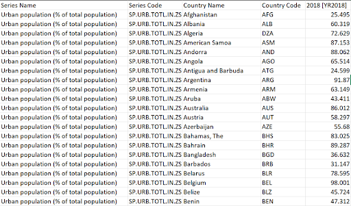
- Ratio of urban population to total population (%)
- School enrolment (% of population)
- Public spending on education, total (% of GDP)
- Population, total
- Population Growth (%)
- Life expectancy at birth, total (years)
- Female labour force (% of total labour force)
- GNI per capita, Atlas method (current USD)
- Size of Manufacturing sector (% of total GDP)
- GDP growth (%)
Methodology
We used Jupyter Notebook and Python for data cleaning, and then Python and R packages to analyse our data and create data visualisations.
Our first objective was cleaning and merging multiple datasets coherently. During the merging process, we ensured that the list of countries in both datasets matched each other, such that development data was correctly matched to a country’s PM2.5 concentration. Then, we cleaned the columns of the dataset by eliminating the development indicators with too much missing data. We cleaned the rows of the dataset by using the dropna() function, which enabled us to efficiently get rid of countries with missing values. We also converted data types where applicable. The dimensions of our main dataframe went from 196 rows by 20 columns to 175 rows by 17 columns. The number of rows are the number of countries, and the number of columns is the sum of our 6 remaining development indicators, and yearly PM2.5 concentration between 2010-2019.
Then, the first part of our research looked at the relationship between PM2.5 concentration and individual development indicators. This involved using a multi-linear quadratic log regression model. Using R, we created scatterplots of PM2.5 concentration against each development indicator. We used a logarithmic scale on certain indicators to increase the legibility of our data. We used the stat_smooth function to add a locally weighted polynomial regression (LOESS) to the data. We also created animated plots using panel data over 2010-2019, focusing on the behaviour of key economies at different stages of development.
The second part of our research involved using Principal Component Analysis to create a “development index” using the first principal component. Using PCA is a useful tool to reduce the dimensionality of datasets and create 2D visualisations. In our case, we used the first principal component as a proxy for development, as features of all 6 indicators could be combined into 1 “index”. We then plotted PM2.5 concentration level against the first principal component and added a polynomial regression line.
Obtaining Data
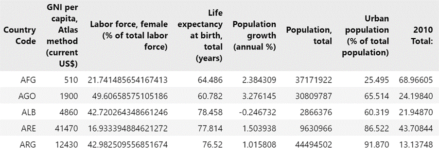
The WHO (World Health Organization) provides yearly PM2.5 concentration data between 2010-2019. The pollution indicator code is SDGPM25, and the data is split across country (SpatialDIM) and across time (TimeDim). Within each country, air pollution is split in 5 categories: “Total”, “City”, “Rural”, “Town” and “Urban”. The data corresponds to population weighted annual mean levels of PM2.5 concentration, measured in μg/m^3. Figure 1 show the raw PM2.5 dataset and a snippet for one country (Afghanistan) and one year (2010). We wanted to do cross country comparisons, so we chose to look at “Total” concentration over 10 time periods for all 195 countries. We chose “Total” because this makes for more accurate comparisons between countries as each country has a different composition of urban and rural areas.
Fig 2 show the raw PM2.5 dataset and a snippet for one country (Afghanistan) and one year (2010).
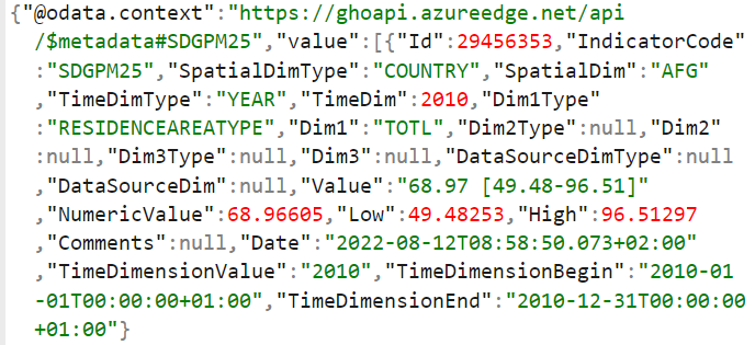
We then checked the values we got with the original json file, and realized they were incorrect. We then checked for missing data values and found that with 9450 data points and 195 countries, there were less than 50 data points per country, which meant there was some missing data since each country had 5 locations over 10 years. We then went back to the documentation for the API and through trial and error (since the documentation was very vague) found a way to filter for just the total values for each country which didn’t have missing data in it. As such, using the list comprehension tool and vectorised operations through the pandas library, we also made our code faster.
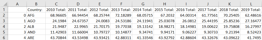
This resulted in the following dataset (196 rows * 11 columns):
For the development indicators, we downloaded data from the World Bank’s database as a CSV file and cleaned the data on python.
Data Wrangling
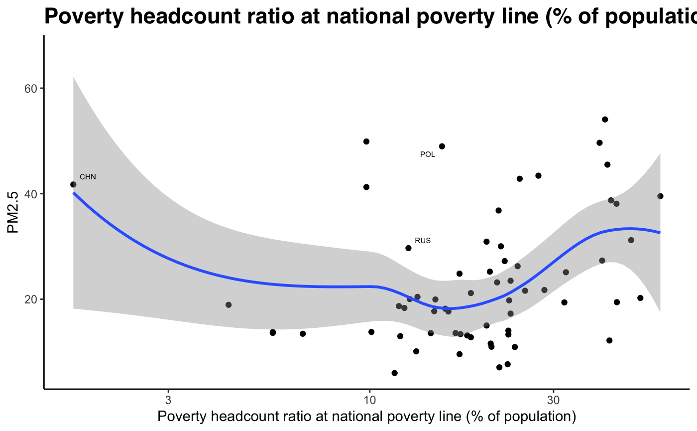
We realised that 4 of our indicators (School Enrolment, Public Spending on Education, Poverty headcount ratio, size of manufacturing sector) had less than 100 datapoints (out of 195 countries), so keeping them would mean working with a much smaller pool of countries. This could also bring bias into our data, as low income countries are generally more likely to have missing data than high income countries. As such, we reduced the number of development indicators from 10 to 6. With these, we dropped countries with missing values across the indicator list, reducing the number of countries from 195 to 175. As shown above, the development dataset was in ‘long’ format. Merging with the air pollution dataframe enabled us to change the dataset to ‘wide’ format. We used the df.merge (on) function to merge both datasets on “country code”.
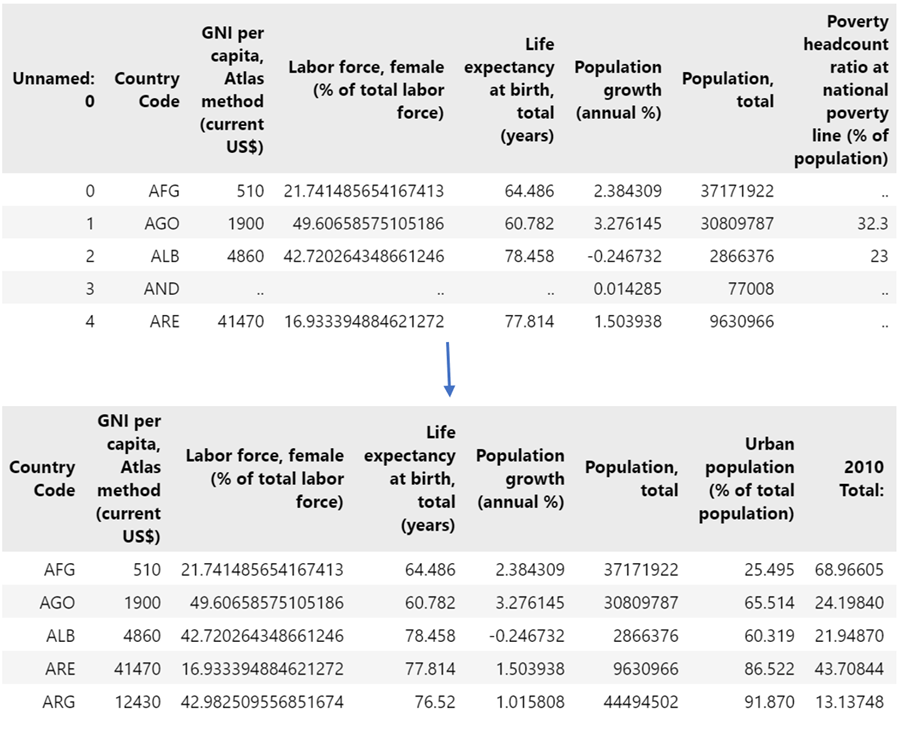
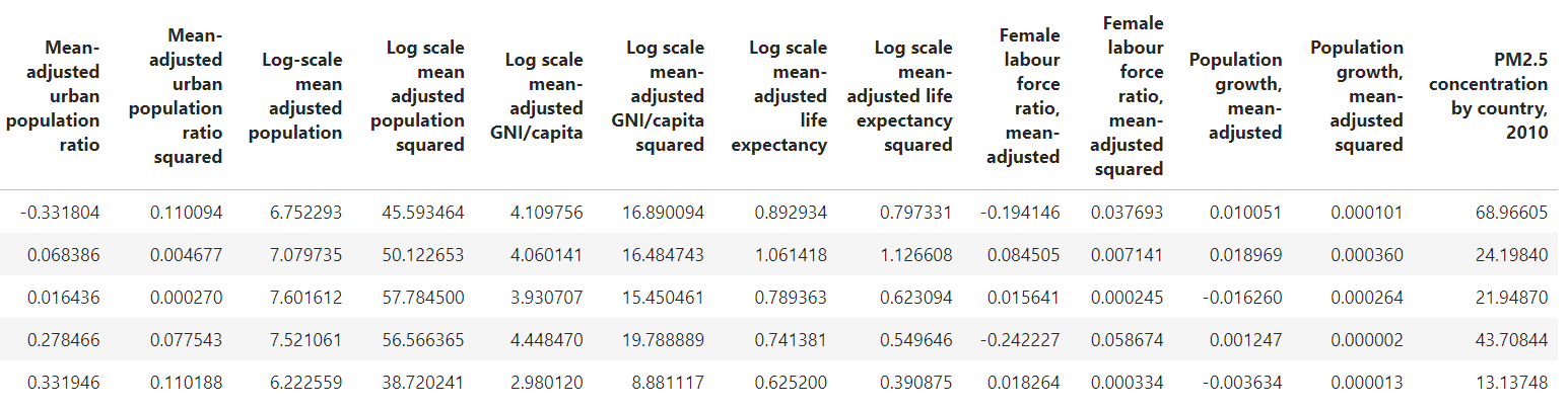
As such, our final dataframe was 175 rows by 17 columns, which we could then use to carry out data visualisations:
Main Limitations:
- Our primary analysis only focuses on PM2.5 concentration levels over a short time period (2010-2019), which are the limits of the WHO’s PM2.5 data. Since changes in economic development typically occur over longer time periods, our research would have benefited from having access to historical PM2.5 data (e.g. 1980-).
- For simplicity, we chose to ignore the countries with missing data (NaN values) and indicators with too much missing data. This may introduce bias into our data, as low income countries may have disproportionately more missing data than high income countries. As shown in Angrist et al. (2021), “limited statistical capacity, the use of outdated data and methods, the large share of the agricultural sector, the informal economy and limited price data” are potential reasons why. However, our data cleaning only reduced the scope of countries by 20, going from 195 to 175 countries.
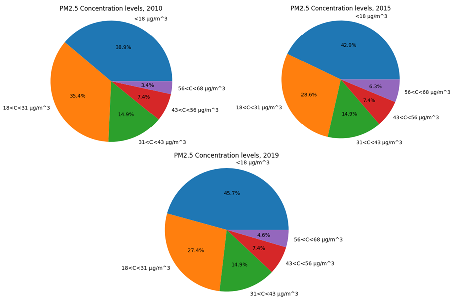
- For the PCA analysis, we used data from a single year (2018) to generate a plot of PM2.5 concentration against development level. This might make our model inaccurate: if 2018 was an “outlier” year for multiple countries, then this could distort the shape of our Kuznets curve. Hence, we replicated our plot using PM2.5 data from 2010, 2015 and 2019.
- Our data does not take account for income inequality, which can be factored into determining a country’s economic development. Thus, in very unequal societies, GNI/capita may overstate the level of economic development, which could reduce the accuracy of our development index.
Exploratory data analysis:
We started by looking at changes in the distribution of PM2.5 concentration over time.
![Fig. 4: Distribution of world PM2.5 concentration data [175 countries] across time.](visualisations + webpage pictures\boxplot_NEW.png)
As the boxplot shows, between 2010 and 2019, PM2.5 across the world have stayed at similar levels. Median air pollution has declined from 21.3 μg/m^3 to 18.8 μg/m^3. The standard error increased from 1.05 to 1.11 between 2010 and 2015, but declined again to 1.04 in 2019.
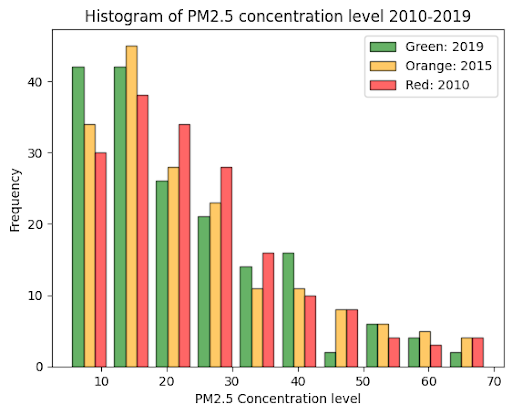
The histogram above shows the change in the distribution of PM2.5 levels across classes. Between 2010 and 2019, more than 10 countries reduced their PM2.5 levels below 10 μg/m^3. At the other tail of the distribution, countries with very high PM2.5 levels have seen a decline in their pollution levels, shifting towards the middle of the distribution.
Geographically, most of the countries with high PM2.5 concentration are Asia, the Middle East and Sub-Saharian Africa. Those with low levels of PM2.5 concentration tend to be more economically developed countries, since they have implemented policies to reduce emissions and pollution levels for much longer. For example, nearly all countries in Europe, as well as the US and Canada have below 25 µg/m^3 PM2.5 concentration. Countries with low population density, such as Russia and Austrialia also have low PM2.5 levels. On the other hand, countries with complex topography, as well as high population density, tend to have higher pollution levels. For example, Afghanistan has one of the highest levels in PM2.5. Egypt, with a high population density around the Nile Valley, also has high PM2.5 levels. Lastly, countries with carbon intensive energy production, such as power stations in China and oil refineries in Nigeria, tend to see high levels of PM2.5 concentration.
Results
Sub-Problem 1: Which development indicators best predict a U-shaped Environmental Kuznets Curve?
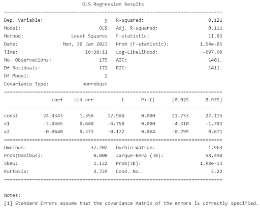
We used the LinearRegression package on Python to find the most significant development indicators using a quadratic regression model.

Description of regression variables:
X_1 = Share of urban population, mean-adjusted
X_2 = Log population, mean-adjusted
X_3 = Log Life expectancy, mean-adjusted
X_4 = Log Life expectancy, mean-adjusted
X_5 = Female labour force ratio, mean-adjusted
X_6 = Population growth, mean-adjusted
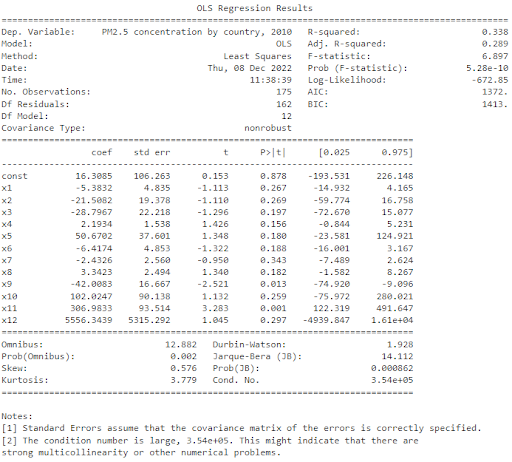
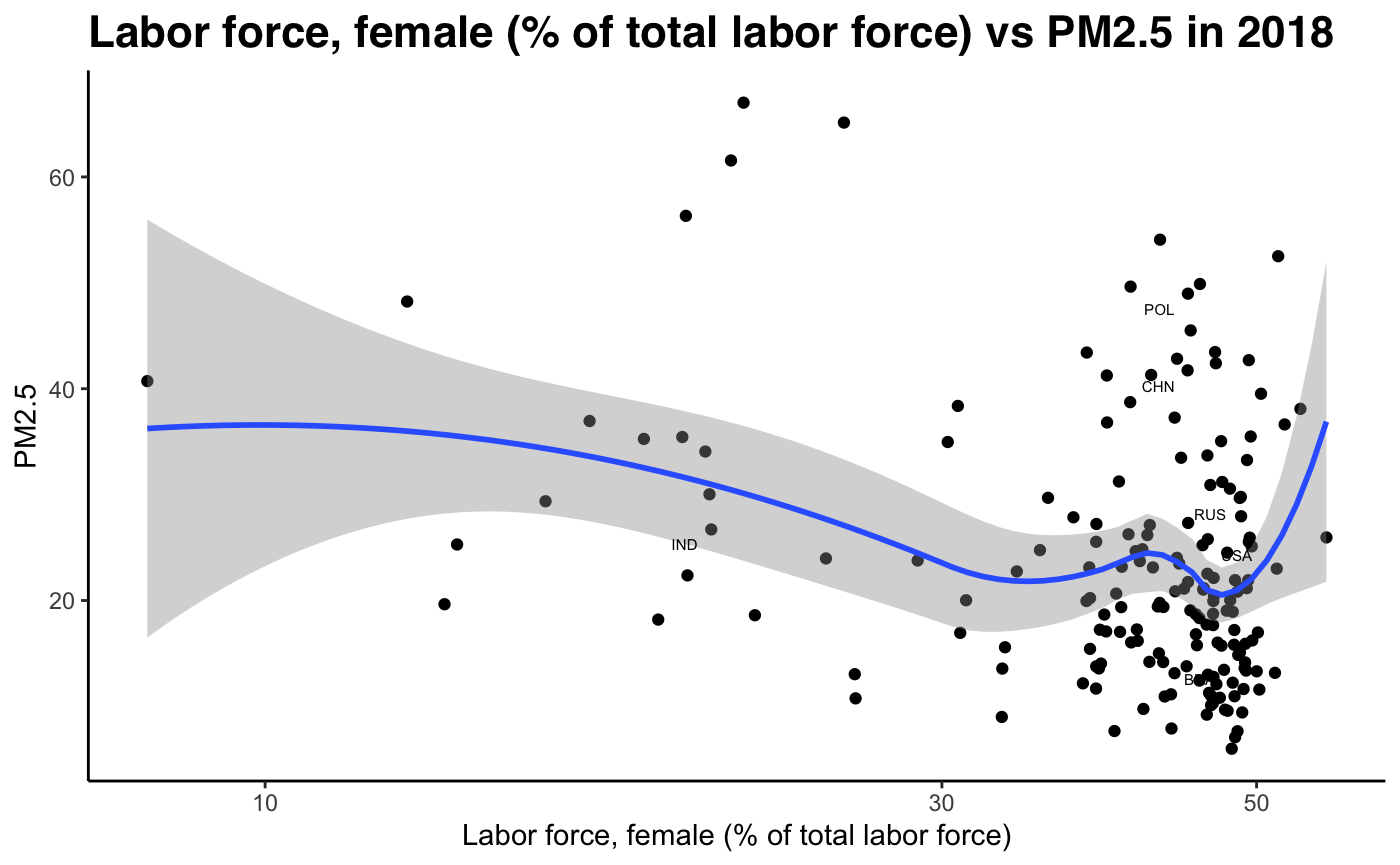
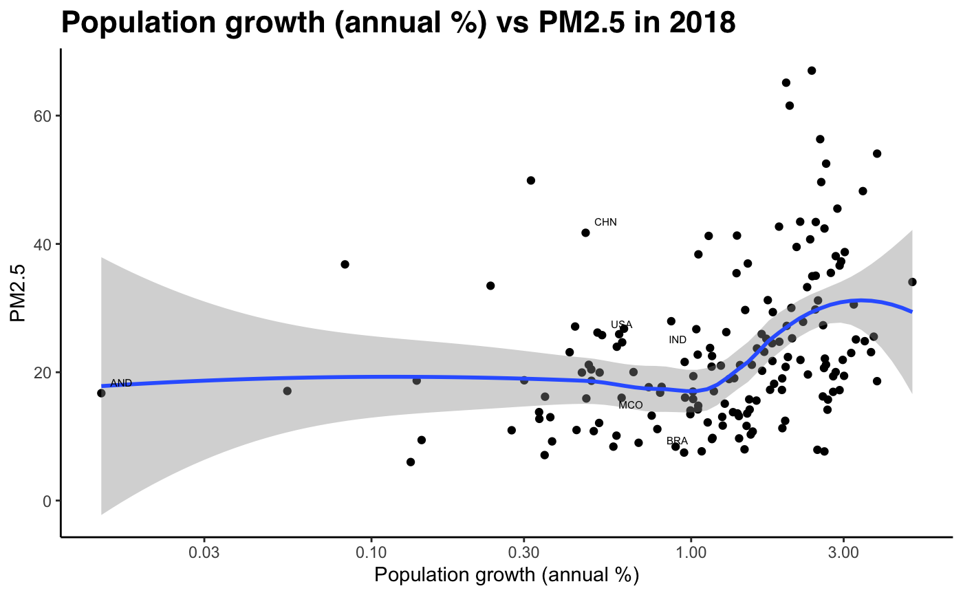
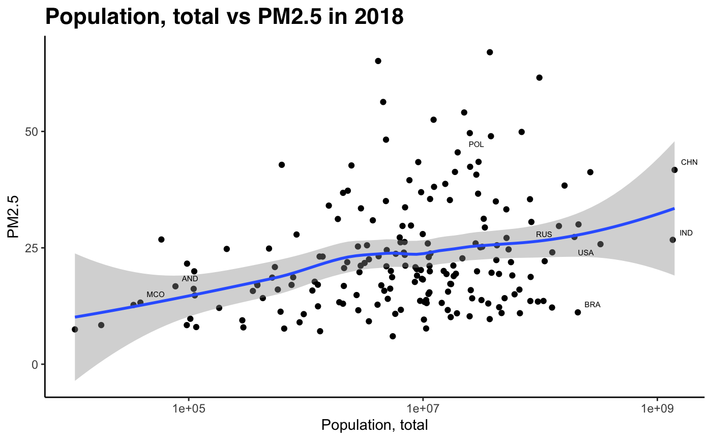
As shown by the table of regression results, the variables which stand out most are the linear terms of X_5 (p=0.013) and X_6 (p=0.001). These correspond to population growth (x11), and female labour force ratio (x9). For quadratic terms, the most relevant indicators are log population (x4), log GNI/capita (x6) and log life expectancy (x8).
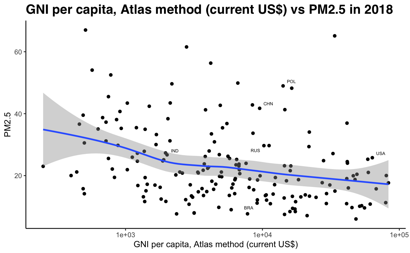
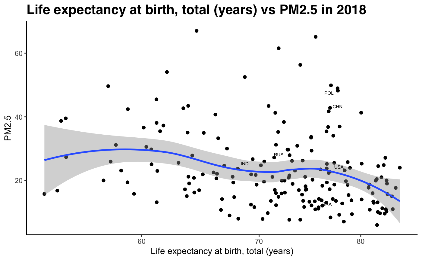
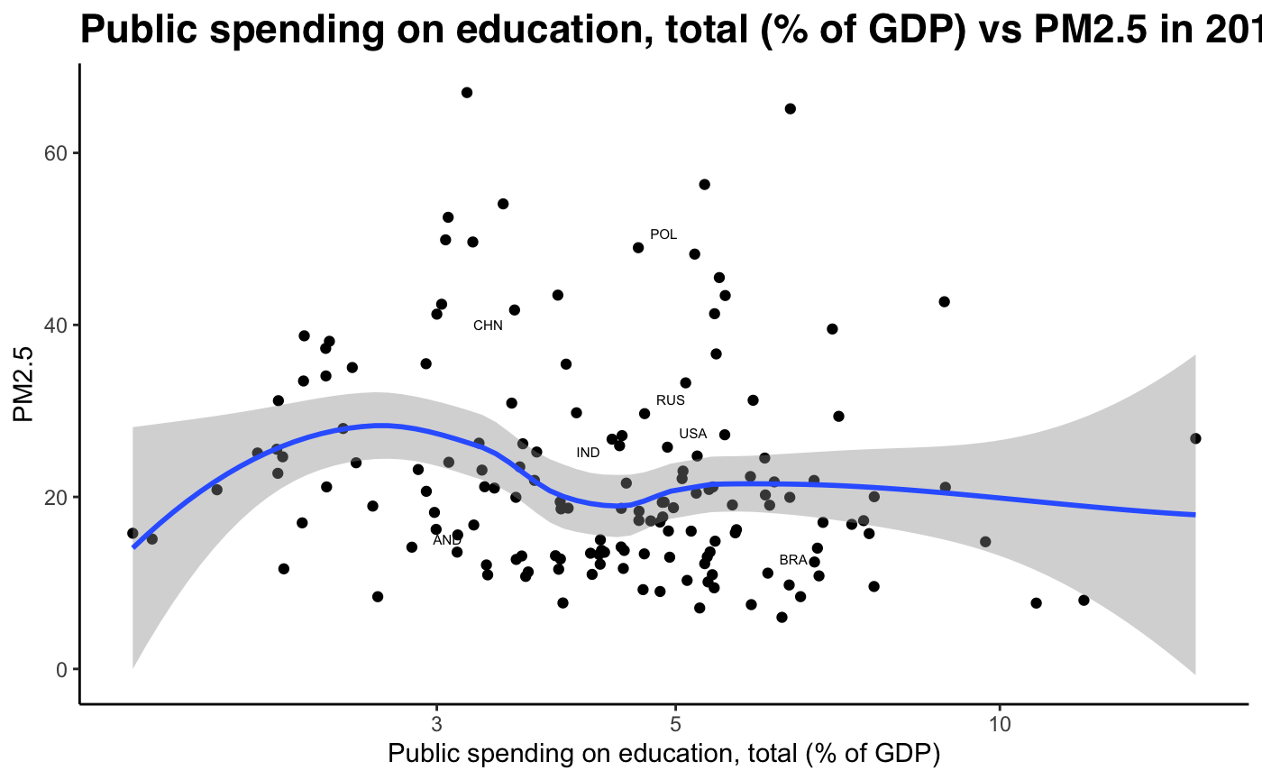
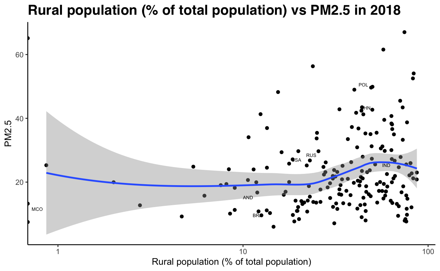
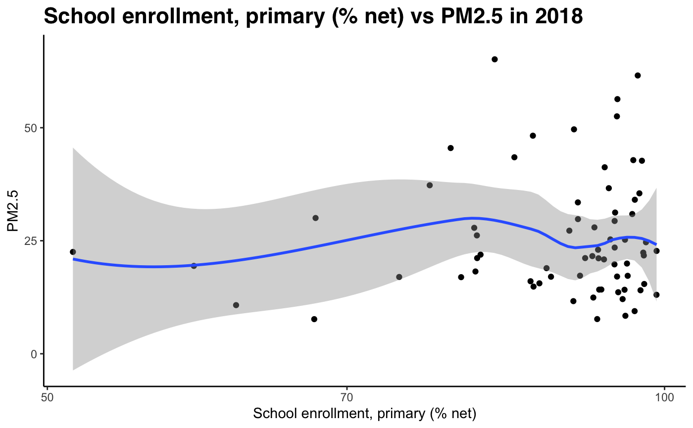
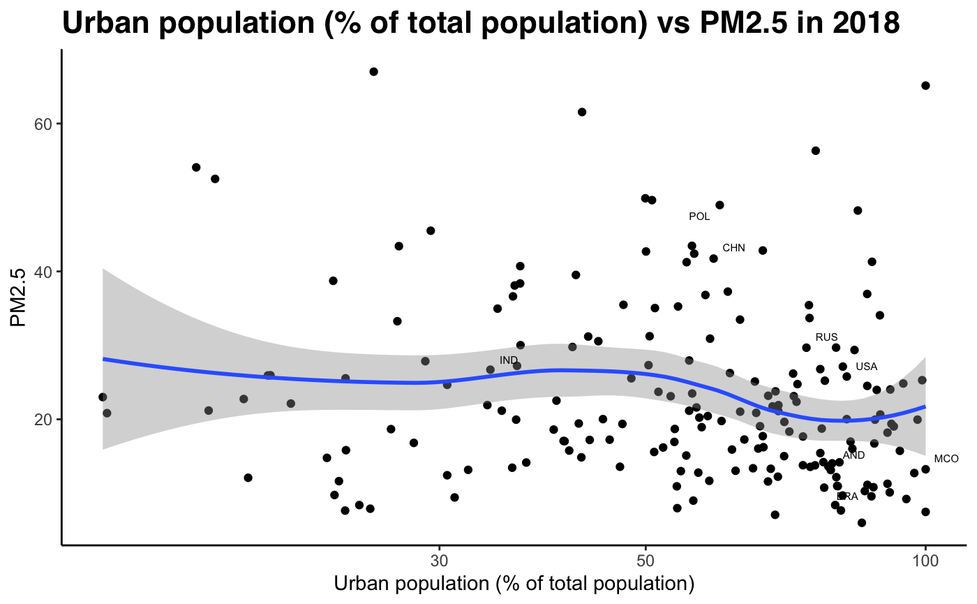
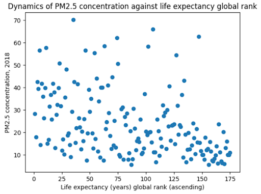
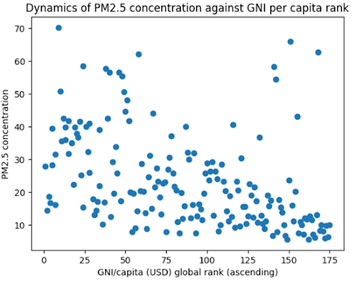
By looking at GNI/per capita data against PM2.5 data, we can see that pollution levels decline at early stages of development, as economies experience booming economic growth. This runs contradictory to the expected shape of the Kuznets curve, which predicts increasing emissions up to full industrialisation. The only key indicator which seems to show some validity to the Kuznets curve is life expectancy. As life expectancy increases, the level of development increases, and for early-development economies we see a slight increase in pollution levels. However, we observe a twin-peak, where pollution levels seems to rise again when life expectancy levels are around 75 (most of the data points). At the right tail, we see a more pronounced decrease in PM2.5 concentration levels once life expectancy hits 80+ years. This is a sign of high income developed economies.
Fig 12-21: PM2.5 concentration against develpment indicators, 2018
Sub-Problem 2: How well does our hypothesis hold using our development index (PCA)?
We used Principal Component Analysis (PCA) to reduce the dimensionality of our dataset from n=6 to n=2. Inputting 6 variables returns 6 principal components, each showing a linear combination of the 6 variables. Each principal component represents the “direction vector” of the maximal amount of variance in the dataset. Therefore, all principal components will be orthogonal to each other, and we can select the first principal component, which retains most information about the data.
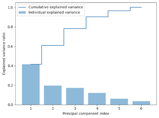
The explained variance of the first principal component was 0.414, the second 0.195, the third 0.172 and so on. The first principal component is “best” as it encapsulates the most information about the variance in the data.
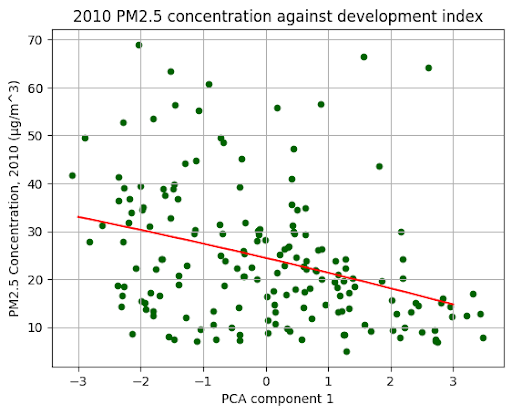
As shown above, fitting a polynomial regression of degree 2 (since the Kuznets curve has a quadratic shape) to our plot showed a weak correlation between our first principal component and PM2.5 concentration. We then used the Linear Regression package in sklearn to confirm our results. x1 was PC1, and x2 was PC1^2 (the quadratic term). Whilst x2 had a weak p-value, x1 had a p-value < 0.05, which implied a negative linear relationship between PM2.5 and our development index, as witnessed on the scatter plot.
Sub-problem 3: What can we learn from using panel data?
We decided to zoom in and look at the relationship between Population growth % vs PM2.5 and GNI vs PM2.5 over time between 2010-2019. To visualise our data, we used ggplot2 and gganimate packages to create dynamic plots. In order to enhance comprehension of the patterns over time in Brazil, we opted to include labels specifically for the country. Our focus on Brazil allowed us to delve deeper into the country's evolution.
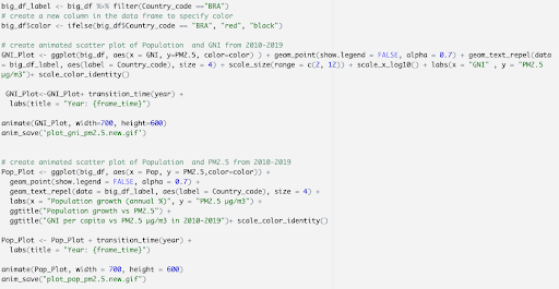
Our analysis reveals that while a few countries exhibit substantial fluctuations over time, the majority show relatively stable patterns. Upon closer examination of Brazil, we were unable to observe the U shaped pattern described by the Environmental Kuznets Curve.