BRAZIL ANALYSIS

Motivation

Because we found limited evidence of the Environmental Kuznets Curve when making cross-country comparisons, we wanted to investigate the issue further. One of the potential reasons for not seeing the curve is that countries have different characteristics that could impact PM2.5 concentration through channels other than development. There may be country fixed effects that we do not account for. We specifically choose to focus on Brazil, because it went through different stages of development in a relatively short time. This would allow us to cover a large span of development, with fewer data, which is useful since PM2.5 data is not available on a large time horizon.

Initially, we wanted to do a times series analysis of the data, to assess the strength of the relationship between PM2.5 and economic development, measured by GDP/capita. However, since there is limited data on historical PM2.5, we decided against continuing with the time series analysis.

When researching empirical literature, we came across a paper on the relationship between PM2.5 and economic development in China. The authors used a Spatial Durbin model to examine the relationship between PM2.5 data and economic growth in 13 cities of the BTH region from 1998 to 2016 (see appendix). We chose to look at city-level data across different regions in Brazil since there are significant variations in development across the country.

Data used:

For the intertemporal analysis of Brazil:

1. Economic development: Since in the PCA, GDP was a strong indicator, we used the IMF API to collect GDP/capita data on Brazil from 1980-2021. We used the World Bank API to gather data on PM2.5 concentration, which includes data for 1990, 1995, 2000, 2005, 2010-2017.
2. PM2.5: We used the World Bank API, which we also used in the first part of the research.

Data Wrangling:

Intertemporal analysis:

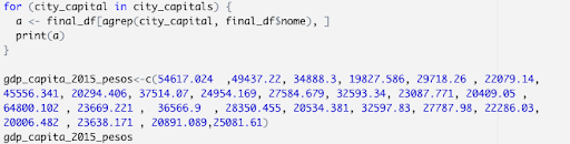
Below is an example of the call used to get the GDP/capita data,and PM2.5 data. We merged the data frames by date so that we can use them to create visualisations as well as scatterplots.

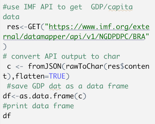
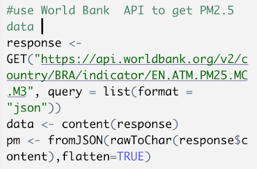
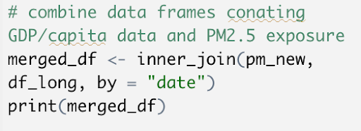
Fig 22: Data extraction from the IMF/World Bank API

Results

We used ggplot2 in R, to create scatter plots that would allow us to visualise the relationship between the variables of interest, GDP/capita and PM2.5, across time.

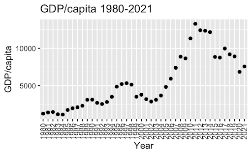
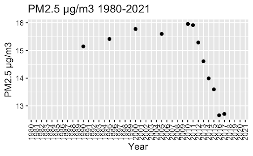
Visually, we are unable to infer a EKC relation. For the time period where GDP/capita is increasing (1980-2011) we see limited increases in PM2.5 from 15 to 16 µg/m^3. For the timer period where GDP/capita decreases we actually also saw a decrease in PM.5 from around 16 to 13 µg/m^3. This would be a linear relation, rather than a curved relation.

However, since there is not enough data available for PM2.5, we were unable to continue with our initial time series analysis. We would essentially only have 12 observations, so a time series regression would not tell us much about the trend. Moreover, PM2.5 data is likely to be auto-correlated from one period to the next. These issues would induce significant bias and could result in spurious correlation results. Therefore, we ultimately decided against doing a time series since it would likely not result in meaningful conclusions about the EKC.

City-level Analysis

Data:

1. PM2.5- We used data from the Socioeconomic Data and Applications Center (SEDAC2), presented as annual global surface concentrations (mi- crograms per cubic metre, mg/m3) of mineral dust and sea-salt filtered PM2.5 over the period of 1998-2016. The data set contains information on 770 Brazilian cities. Of these Brazilian cities, we selected a random sample of 30 cities.
2. Economic development: We choose to focus on GDP/capita since there is no municipality level data on the other development indicators used in the first part of our research.We used the Basedosdados data set to extract municipality level “GDP,” “ID names” and population at the municipality level
3. Cities: We choose to focus on the 26 regional capitals,since they are spread across Brazil so this minimises the effects of PM2.5 spreading across cities. Moreover, they are spread across a range of economic development, minimising the changes that we get cities from only one side of the curve.

Data Wrangling

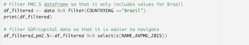
To get city level PM2.5 data we filtered the data set to only include values for Brazil, and selected only the relevant columns on city name and year 2015.

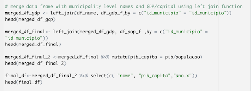
To get municipality level GDP/capita we had to combine three data sets, since the “GDP”, “population” and “municipality id” were in separate data frames.

To get the ‘capital cities’ dataset, we manually imputed the names of the cities.

The Basedosdatos data set contains GDP/capita figures but they are inaccurate, so we had to divide municipality GDP by the municipality population.

We encountered difficulties when trying to match the data sets, since the city names in the GDP/capita and PM2.5 datasets are spelled differently. As such we had to use fuzzy match. However, since the results returned were not perfect we had to manually create a data set.

The insert shows an excerpt of the final data frame:

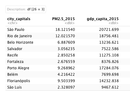
This process was manageable since we chose to focus on the key cities, but it limits the possibility of extending the research to the whole data set of 770 cities. Moreover, one of the cities did not have PM2.5 data which induced missing data in our analysis at a capital city level.

Results

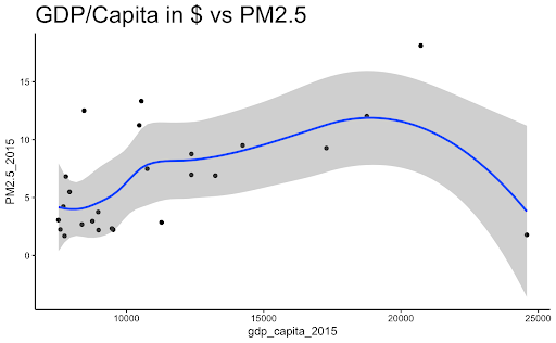
The scatterplot below shows the relationship between GDP/capita and PM2.5 in 2015. We used the stat_smooth function to add a locally weighted polynomial regression (LOESS) to our scatterplot. We can see that the data displays more of the expected U-shaped relation, which corresponds to a greater extent to the relationship implied by the EKC. We can see that cities that have higher levels of GDP have lower levels of PM2.5 pollution. However, we can also see that at lower levels of development, PM2.5 levels span from about 2 to 15 µg/m3. Therefore, further investigation would be necessary in order to grasp the full effects.

Conclusion

In this research project, we aimed to use both macro-level and micro-level data to display a U shaped relationship between air pollution levels and PM2.5, as shown by the Environmental Kuznets curve. To do so, we conducted cross-country and city-level comparisons by plotting different development indicators against PM2.5 levels for 175 countries. Our findings showed little evidence of the U shaped relationship implied by the EKC. Instead, we found that key development indicators only went so far in predicting a bell shaped pattern for PM2.5. Our PCA model showed that PM2.5 concentration tended to decrease as the level of development (measured by our development index) increased. Since widespread measurement of PM2.5 concentration is relatively new, the lack of historical data meant that we could only draw limited conclusions about the evolution of PM2.5 levels over time. Our city-level analysis focused on Brazil, where we conducted a spatial analysis of the relationship between GDP/capita and PM2.5 in key Brazilian cities. Our results showed that even at the micro-level, evidence of the Kuznets curve relation was hard to discern.

However, our research also shows optimistic trends in reducing air pollution across the globe. In just the last 10 years, the number of countries achieving low levels of PM2.5 concentration has increased. Meanwhile, countries with very high air pollution levels have seen declines in their pollution levels. On the whole, a fine balancing act between economic growth and environmental protection is needed to ensure a smooth transition

What could be next?

The climate crisis is a crucial issue that demands our immediate attention, and to tackle it effectively, we need to have a deep understanding of the factors that can drive sustainable environmental change. To gain a more complete picture of the Environmental Kuznets Curve dynamics, we recommend extending our research efforts. Specifically, by continuing our spatial analysis of Brazilian cities and incorporating multiple years of data, we can conduct a temporal spatial analysis to better understand the relationship between economic development and PM2.5. We could also extend our analysis to different types of pollutants such as social and water pollutants. This will provide valuable insights that could inform the development of effective policies aimed at protecting the environment.

Appendix

Data Sources

1. PM2.5 air pollution, mean annual exposure (micrograms per cubic meter) | DATA
2. IMF DataMapper API documentation
3. Base dos Dados
4. SEDAC Releases Air Quality Data for Health-Related Applications | Earthdata

Kuznets curve background research:

1. Alstine, J. V., & Neumayer, E. (2010). The environmental Kuznets curve. In K. P. Gallagher, Handbook on trade and the environment (pp. 49-59). Cheltenham UK.

2. Grossman, G. M., & Krueger, A. B. (1995). Economic Growth and the Environment. The Quarterly Journal of Economics, 110(2), 353–377.

3. Taguchi, H. (Apr 2013,). The environmental kuznets curve in Asia: The case of sulphur and carbon emissions. Asia-Pacific Development Journal, Volume 19, Issue 2, , p. 77 - 92.

4. Ding, Y., Ming, Z., Chen, S., Wang, W., Nie, R., “The environmental Kuznets curve for PM2.5 pollution in Beijing-Tianjin-Hebei region of China: A spatial panel data approach” (2019)

Back: